January 1, 0001
This dataset analyzes 79 urine samples to see if there is a relationship between certain physical characteristics of the urine and the formation of calcium oxalate crystals. There are seven variables in this dataset, out of which one is binary and the others are numeric. The variables are r, gravity, pH, osmo, cond, urea, and calc representing the presence of calcium oxalate crystals, the specific gravity of the urine, the pH reading of the urine, the osmolarity of the urine, the conductivity of the urine, the urea concentration in millimoles per litre, and the calcium concentration in millimoles per litre, respectively.
1. MANOVA testing
manova1 <- manova(cbind(gravity, ph, osmo, cond, urea, calc) ~ r, data = urine)
summary(manova1)
## Df Pillai approx F num Df den Df Pr(>F)
## r 1 0.42205 8.5197 6 70 5.933e-07 ***
## Residuals 75
## ---
## Signif. codes: 0 '***' 0.001 '**' 0.01 '*' 0.05 '.' 0.1 ' ' 1A one-way multivariate analysis of variance (MANOVA) was conducted to test the effect of the smoking or not smoking (variable = smoke) on six dependent, numeric variables: the specific gravity of the urine (gravity), the pH reading of the urine (ph), the osmolarity of the urine (osmo), the conductivity of the urine (cond), the urea concentration in millimoles per litre (urea), and the calcium concentration in millimoles per litre (calc). Significant differences were found for presence of calcium oxalate crystals for all six dependent, numeric variables. The p-value is 5.933e-07 and since it is less than 0.05, there is a significant mean difference across levels of the categorical variable. MANOVA assumptions are
summary.aov(manova1)## Response gravity :
## Df Sum Sq Mean Sq F value Pr(>F)
## r 1 0.0007277 0.00072771 16.359 0.0001259 ***
## Residuals 75 0.0033362 0.00004448
## ---
## Signif. codes: 0 '***' 0.001 '**' 0.01 '*' 0.05 '.' 0.1 ' ' 1
##
## Response ph :
## Df Sum Sq Mean Sq F value Pr(>F)
## r 1 0.742 0.74233 1.4319 0.2352
## Residuals 75 38.883 0.51844
##
## Response osmo :
## Df Sum Sq Mean Sq F value Pr(>F)
## r 1 277091 277091 5.0919 0.02695 *
## Residuals 75 4081331 54418
## ---
## Signif. codes: 0 '***' 0.001 '**' 0.01 '*' 0.05 '.' 0.1 ' ' 1
##
## Response cond :
## Df Sum Sq Mean Sq F value Pr(>F)
## r 1 13.0 12.953 0.2 0.656
## Residuals 75 4856.1 64.748
##
## Response urea :
## Df Sum Sq Mean Sq F value Pr(>F)
## r 1 92220 92220 5.7551 0.01893 *
## Residuals 75 1201808 16024
## ---
## Signif. codes: 0 '***' 0.001 '**' 0.01 '*' 0.05 '.' 0.1 ' ' 1
##
## Response calc :
## Df Sum Sq Mean Sq F value Pr(>F)
## r 1 240.81 240.812 30.859 4.031e-07 ***
## Residuals 75 585.28 7.804
## ---
## Signif. codes: 0 '***' 0.001 '**' 0.01 '*' 0.05 '.' 0.1 ' ' 1
##
## 2 observations deleted due to missingnessTo follow up on the manova, univariate ANOVA tests were performed for each dependent variable, as shown below. Of the numeric variables, the p-values were less than 0.05 for osmo (p-value is 0.02695), urea (p-value is 0.01893), calc (p-value is 4.031e-07), and gravity (p-value is 0.0001259), indicating that these four numeric values show a significant mean difference across r. Numeric variables, cond (p-value is 0.656) and ph (0.2352), have p-values greater than 0.05 indicating that that these two do not show a significant mean difference across r.
1-(0.95^7) #probability of atleast one type 1 error## [1] 0.3016627#0.3016627
0.05/7 #bonferri correction## [1] 0.007142857#0.007142857Since the categorical predictor has two levels and the ANOVAs already tell us that the two groups differ, the post hoc t-tests are not needed. 1 MANOVA and 6 ANOVAs were performed for a total of 7 tests. The probability of a Type 1 error is 30.17 percent. The value of Bonferroni’s correction is 0.007142857. With the significance level adjusted to this, the new numeric values with p-values less than this showing a significant mean difference across r are calc (p-value is 4.031e-07) and gravity (p-value is 0.0001259).The assumptions of a MANOVA test are multivariate normality of dependent variables, independent sample and random observations, homogeneity of covariance matrices, and linear relationships between dependent variables, and no extreme univariate or multivariate outliers, no multicollinearity. These assumptions have to be met for a successful MANOVA, which we were able to perform.
2. Randomization Test
t.test(data=urine,osmo~r)##
## Welch Two Sample t-test
##
## data: osmo by r
## t = -2.2095, df = 69.391, p-value = 0.03044
## alternative hypothesis: true difference in means is not equal to 0
## 95 percent confidence interval:
## -223.75096 -11.42884
## sample estimates:
## mean in group 0 mean in group 1
## 565.2889 682.8788t.test(data=urine,cond~r)##
## Welch Two Sample t-test
##
## data: cond by r
## t = -0.45723, df = 75.983, p-value = 0.6488
## alternative hypothesis: true difference in means is not equal to 0
## 95 percent confidence interval:
## -4.316287 2.704522
## sample estimates:
## mean in group 0 mean in group 1
## 20.55000 21.35588t<-vector()
for(i in 1:10000){
samp<-rnorm(25,mean=5)
t[i] <- (mean(samp)-5)/(sd(samp)/sqrt(25))
}
data.frame(t)%>% ggplot(aes(t))+geom_histogram(aes(y=..density..), bins=30)+ stat_function(fun=dt,args=list(df=24),geom="line")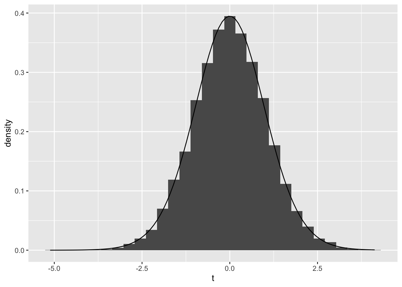 I used the two sample t-test to see whether the averages of the osmolarity of the urine (osmo) and the conductivity of the urine (cond) had significant mean differences when the calcium oxalate crystals formed vs. when they didn’t form. The null hypothesis is that there is no significant difference in the means between osmolarity of the urine (osmo) and the conductivity of the urine (cond) when the calcium oxalate crystals formed vs. when they didn’t form. The alternate hypothesis is that there is a significant difference in the means between osmolarity of the urine (osmo) and the conductivity of the urine (cond) when the calcium oxalate crystals formed vs. when they didn’t form. The first t-test explored the interaction of osmolarity of the urine with the formation of calcium oxalate crystals and had a p-value of 0.0269. Therefore, we accept the null hypothesis and confirm a significant difference in osmolarity of the urine with formation of calcium oxalate crystals. The second t-test explored the interaction of conductivity of the urine with the formation of calcium oxalate crystals and had a p-value of 0.6349, meaning we reject the null hypothesis and that were was no significant mean difference between the interaction of conductivity of the urine with the formation of calcium oxalate crystals. A plot visualizing the null distribution and the test statistic can be seen above.
3. Linear Regression Model (predicting one of the response variables)
urine$gravity_c<- urine$gravity-mean(urine$gravity)
urine$calc_c<- urine$calc-mean(urine$calc)
fit3<-lm(gravity_c ~ calc_c*r, data=urine)
summary(fit3)
##
## Call:
## lm(formula = gravity_c ~ calc_c * r, data = urine)
##
## Residuals:
## Min 1Q Median 3Q Max
## -0.0143001 -0.0045758 -0.0001741 0.0041171 0.0167160
##
## Coefficients:
## Estimate Std. Error t value Pr(>|t|)
## (Intercept) -0.0005850 0.0011822 -0.495 0.62219
## calc_c 0.0013474 0.0004958 2.718 0.00816 **
## r1 0.0024692 0.0016873 1.463 0.14755
## calc_c:r1 -0.0005539 0.0005760 -0.962 0.33934
## ---
## Signif. codes: 0 '***' 0.001 '**' 0.01 '*' 0.05 '.' 0.1 ' ' 1
##
## Residual standard error: 0.006127 on 75 degrees of freedom
## Multiple R-squared: 0.3113, Adjusted R-squared: 0.2838
## F-statistic: 11.3 on 3 and 75 DF, p-value: 3.376e-06#regression plot
ggplot(urine, aes(x=calc, y=gravity,group=r))+geom_point(aes(color=r))+
geom_smooth(method="lm",formula=y~1,se=F,fullrange=T,aes(color=r))+
xlab("calcium concentration (millimoles/L)") + ylab("specific gravity of the urine")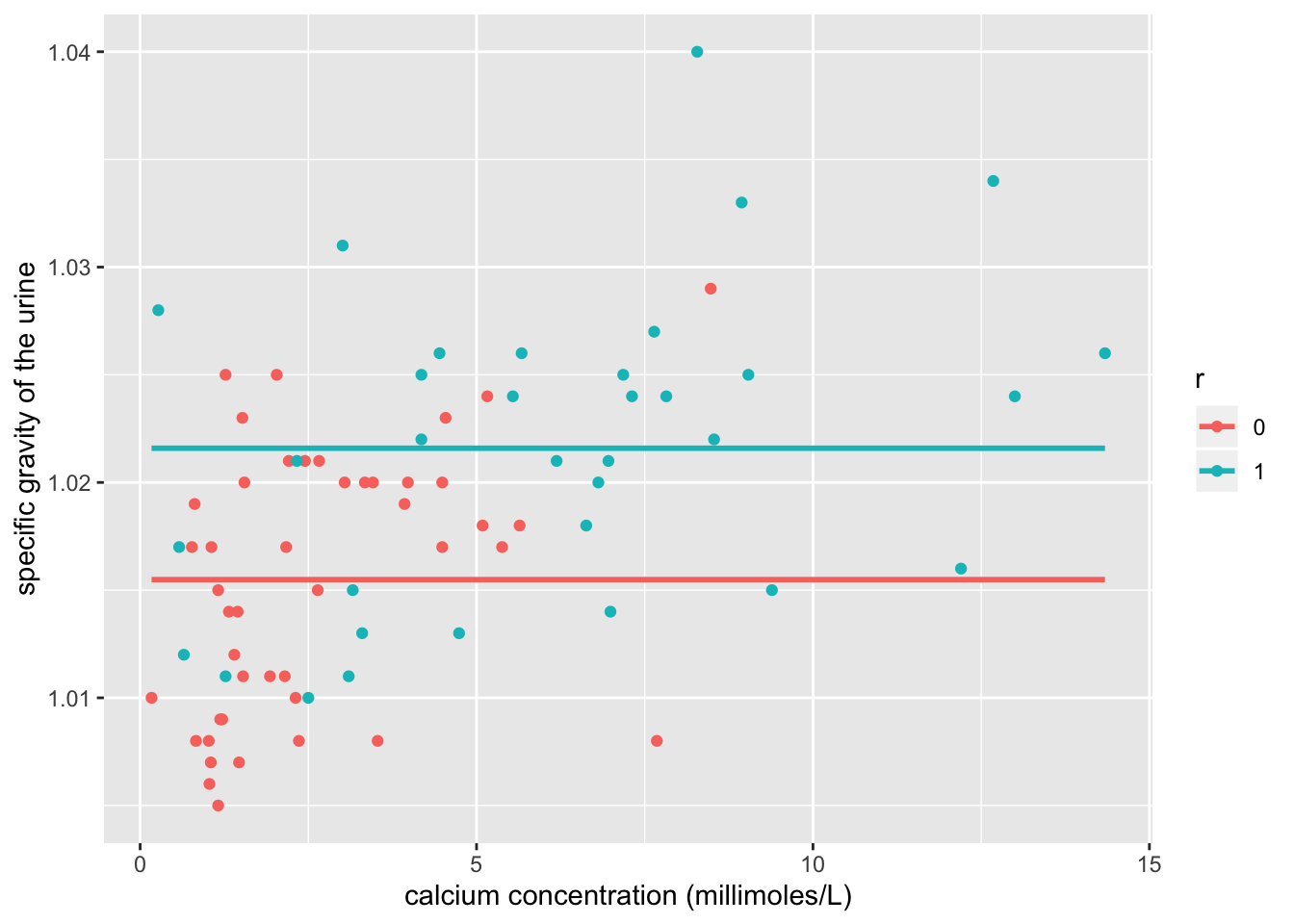
#assumptions (linearity, homoskedsaticity)
resids<-fit3$residuals
fitvals<-fit3$fitted.values
ggplot()+geom_point(aes(fitvals,resids))+geom_hline(yintercept=0, color='yellow')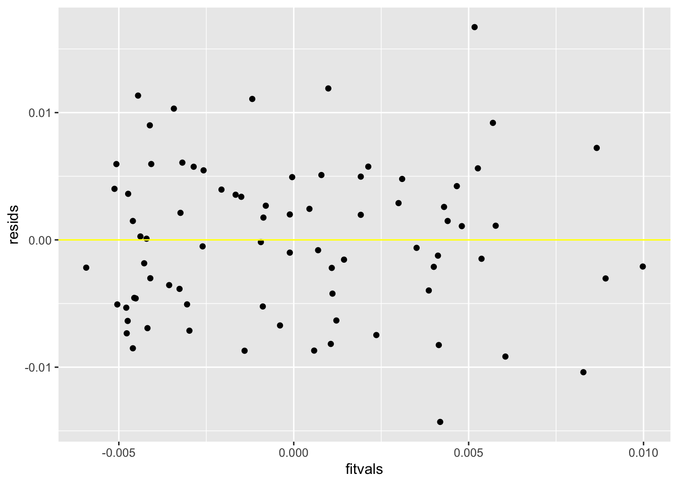
bptest(fit3) #Breuch-Pagan test (null hypothesis: homoskedasticity)##
## studentized Breusch-Pagan test
##
## data: fit3
## BP = 1.7299, df = 3, p-value = 0.6303#With a p-value of 0.6303 (more than 0.05), the null hypothesis can't be rejected and we confirm that heteroskedasticity is not the case in the model. Model is homoskedastic.#assumptions (normality)
ggplot()+geom_histogram(aes(resids), bins=20) 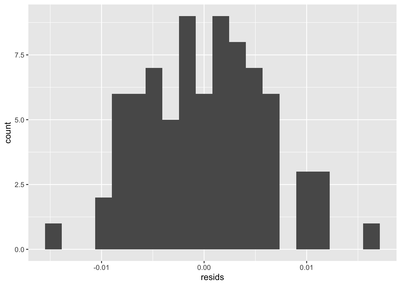
#based off of the histogram of residuals, normality is met. #robust standard errors
summary(fit3)$coef[,1:2] #uncorrected SEs## Estimate Std. Error
## (Intercept) -0.0005849628 0.0011822432
## calc_c 0.0013473842 0.0004957918
## r1 0.0024691544 0.0016873249
## calc_c:r1 -0.0005538931 0.0005760162coeftest(fit3, vcov=vcovHC(fit3))[,1:2] #corrected SE## Estimate Std. Error
## (Intercept) -0.0005849628 0.0015558441
## calc_c 0.0013473842 0.0007127490
## r1 0.0024691544 0.0020880884
## calc_c:r1 -0.0005538931 0.0007968477#The standard errors are slightly higher in the corrected output, however the intercept and coefficient estimates remain the same.#variation
summary(fit3)$r.sq## [1] 0.3113058#The proportion of the variation in the outcome explained by the model is 0.3113058 or 31.13%.fit3rerun <- lm(gravity ~ r+calc, data=urine) #regression without interactions
lrtest(fit3rerun, fit3) #likelihood ratio test## Likelihood ratio test
##
## Model 1: gravity ~ r + calc
## Model 2: gravity_c ~ calc_c * r
## #Df LogLik Df Chisq Pr(>Chisq)
## 1 4 291.98
## 2 5 292.47 1 0.968 0.3252The intercept explains the gravity value when the value of calcium concentration and r is 0. calcium_c explains that if you hold r constant, every 1 point increase in calcium would increase the gravity score by 0.0013473842. R1 explains that if you hold calcium concentration constant, the presence of calcium oxalate crystals will increase the gravity of the urine by 0.0024692 compared to no calcium oxalate crystals. The interaction explains whether the effect of presence of calcium oxalate crystals on gravity differs by calcium concentration. Out of the linearity, heteroskedsaticity, and normality assumptions, not all are met. Looking at the graph, we can see that the linearity assumption is met due to linear relationship between predictor and response variables. Looking at the graph, we can see that heteroskedasticity is not met because the points do not fan out. We can confirm this with the Breusch-Pagan test where we see that the p-value is 0.6303, and a p-value more than 0.05 accepts the null hypothesis that homoskedasticity is met. Based off of the histogram of residuals, normality is met. When the regression was recomputed with robust standard errors via coeftest, the standard errors were slightly higher than in the uncorrected output run previously. 31.13% of the variation in the outcome is explained by the model.
4. Same regression model with Bootstrapped Errors
fit3<-lm(gravity_c ~ calc_c*r, data=urine)
samp_distn <- replicate(5000, {
  boot_dat <- urine[sample(nrow(urine), replace=TRUE),]
  fit4 <- lm(gravity_c ~ calc_c*r, data=boot_dat)
  coef(fit4)
})

samp_distn%>%t%>%as.data.frame%>%summarize_all(sd)
## (Intercept) calc_c r1 calc_c:r1
## 1 0.001301969 0.0005950907 0.001849648 0.0006948474The bootstrapped standard errors for the intercept, calcium concentration, formation of calcium oxalate crystals or not, and the interaction between the two are 0.001308052, 0.0005891642, 0.001900655, and 0.0006786693, respectively. All of these are bootstrapped errors are slightly less than the corrected robust standard errors, and are slightly more than the uncorrected standard errors.
5. Logistic Regression predicting Binary Category Variable
class_diag<-function(probs,truth){
  tab<-table(factor(probs>.5,levels=c("FALSE","TRUE")),truth)
  acc=sum(diag(tab))/sum(tab)
  sens=tab[2,2]/colSums(tab)[2]
  spec=tab[1,1]/colSums(tab)[1]
  ppv=tab[2,2]/rowSums(tab)[2]
  if(is.numeric(truth)==FALSE & is.logical(truth)==FALSE) truth<-as.numeric(truth)-1

  #CALCULATE EXACT AUC
  ord<-order(probs, decreasing=TRUE)
  probs <- probs[ord]; truth <- truth[ord]
  TPR=cumsum(truth)/max(1,sum(truth))
  FPR=cumsum(!truth)/max(1,sum(!truth))
  dup<-c(probs[-1]>=probs[-length(probs)], FALSE)
  TPR<-c(0,TPR[!dup],1); FPR<-c(0,FPR[!dup],1)
  n <- length(TPR)
  auc<- sum( ((TPR[-1]+TPR[-n])/2) * (FPR[-1]-FPR[-n]) )
  data.frame(acc,sens,spec,ppv,auc)
}
#regression and coefficient estimates
logreg <- glm(r ~ gravity + calc + ph, data = urine, family = "binomial")
coeftest(logreg)##
## z test of coefficients:
##
## Estimate Std. Error z value Pr(>|z|)
## (Intercept) -75.35140 50.26767 -1.4990 0.133873
## gravity 72.82358 48.93252 1.4882 0.136686
## calc 0.39113 0.12092 3.2347 0.001218 **
## ph -0.11340 0.40767 -0.2782 0.780883
## ---
## Signif. codes: 0 '***' 0.001 '**' 0.01 '*' 0.05 '.' 0.1 ' ' 1exp(coef(logreg))## (Intercept) gravity calc ph
## 1.884970e-33 4.235230e+31 1.478650e+00 8.927931e-01#regression and predicted probability
logreg <- glm(r ~ gravity + calc + ph, data = urine, family = "binomial")
probs <- predict(logreg, type = "response")
#class diagnostics - accuracy, sensitivity, specificity, and recall (ppv)
class_diag(probs, urine$r) #class diagnostics## acc sens spec ppv auc
## 1 0.7721519 0.7058824 0.8222222 0.75 0.820915#accuracy
#sensitivity
#specificity
#recall (ppv)#confusion matrix
table(predict = probs > 0.5, truth = urine$r) %>% addmargins()## truth
## predict 0 1 Sum
## FALSE 37 10 47
## TRUE 8 24 32
## Sum 45 34 79#accuracy - proportion of correctly classified cases
(36+23)/77## [1] 0.7662338#sensitivity (tpr) - proportion of presence of calcium oxalate crystals correctly classified
23/33## [1] 0.6969697#specificity (tnr) - true negative right; absence of calcium oxalate crystals correctly classified
36/44## [1] 0.8181818#precision (ppv) - positive predicted value; proportion of calcium oxalate crystals classified out of those which are
23/31## [1] 0.7419355#density of log-odds (logit)
urine$logit<-predict(logreg)
urine$r<-factor(urine$r,levels=c(1,0),labels=c("calcium oxalate crystals present", "calcium oxalate crystals absent"))
ggplot(urine,aes(logit, fill=r))+geom_density(alpha=.3)+
geom_vline(xintercept=0,lty=2)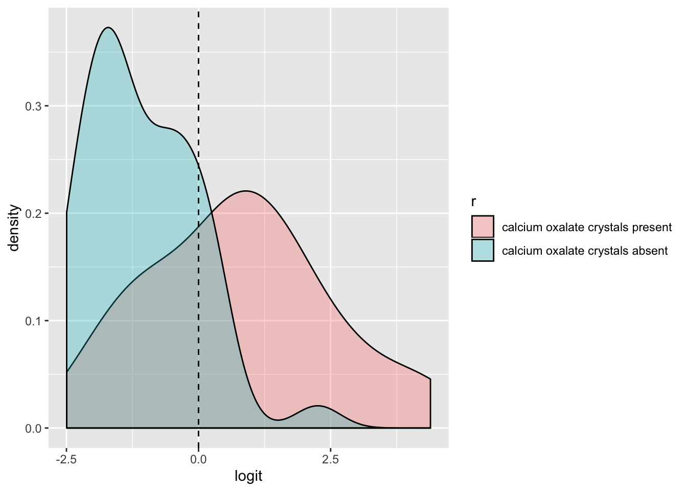
#ROCcurve
ROCcurve<-ggplot(urine)+geom_roc(aes(d=r,m=probs), n.cuts=0) +
  geom_segment(aes(x=0,xend=1,y=0,yend=1),lty=2)
ROCcurve
## Warning in verify_d(data$d): D not labeled 0/1, assuming calcium oxalate
## crystals absent = 0 and calcium oxalate crystals present = 1!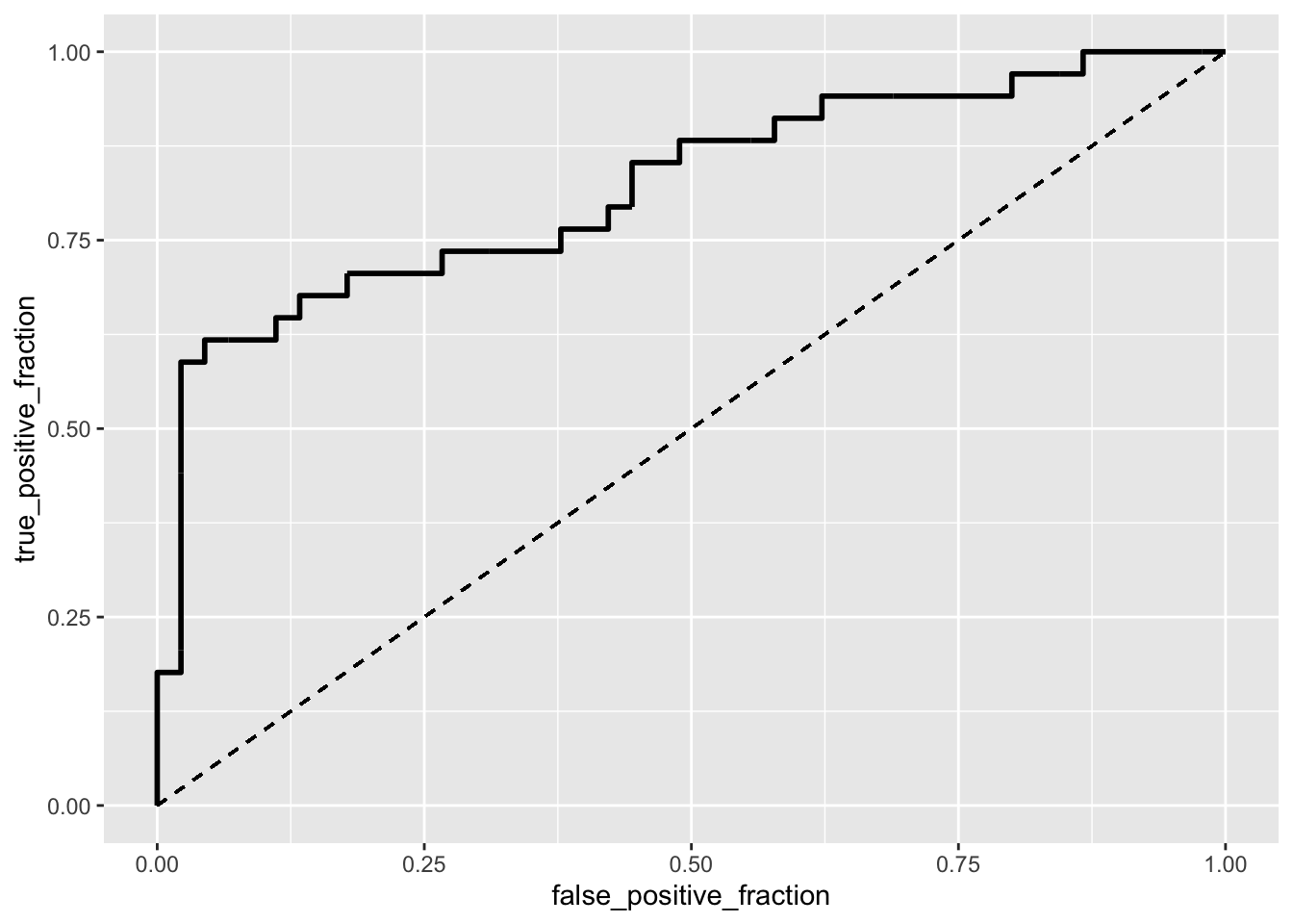
calc_auc(ROCcurve)## Warning in verify_d(data$d): D not labeled 0/1, assuming calcium oxalate
## crystals absent = 0 and calcium oxalate crystals present = 1!## PANEL group AUC
## 1 1 -1 0.820915#The area under the curve is 0.8250689, which is quite good because it's close to 1. #10-fold CV
set.seed(1234)
k=5
data5 <- urine[sample(nrow(urine)), ]
folds <- cut(seq(1:nrow(urine)), breaks = k, labels = F)
diags <- NULL
for (i in 1:k) {
train <- data5[folds != i, ]
test <- data5[folds == i, ]
truth <- test$r
fit5 <- lm(r ~ gravity + calc + ph, data = urine, family = "binomial")
probs5 <- predict(fit5, newdata = test, type = "response")
preds <- ifelse(probs5 > 0.5, 1, 0)
diags <- rbind(diags, class_diag(probs5, truth))
}## Warning in model.response(mf, "numeric"): using type = "numeric" with a factor
## response will be ignored## Warning: In lm.fit(x, y, offset = offset, singular.ok = singular.ok, ...) :
## extra argument 'family' will be disregarded## Warning in Ops.factor(y, z$residuals): '-' not meaningful for factors## Warning in model.response(mf, "numeric"): using type = "numeric" with a factor
## response will be ignored## Warning: In lm.fit(x, y, offset = offset, singular.ok = singular.ok, ...) :
## extra argument 'family' will be disregarded## Warning in Ops.factor(y, z$residuals): '-' not meaningful for factorsapply(diags,2,mean)## acc sens spec ppv auc
## 0.5700000 1.0000000 0.0000000 0.5700000 0.8401293The coeeficient estimates show the effect of the differennt variables on the odds for formation of calcium oxalate crystals. For every one point increase in gravity the odds of calcium oxalate crystals increases by 69.93276. For every one point increase in calcium, the odds of increase by 0.3855. Lastly, for every one point increase in the ph, the odds of calcium oxalate crystals decrease by 0.19867. The accuracy, or the proportion of correctly classified cases, of the model is 0.7662338. The sensitivity, or the proportion of presence of calcium oxalate crystals correctly classified, was 0.6969697. The specificity (tnr), or absensce of calcium oxalate crystals correctly classified is 0.8181818. The recall/ppv/precision, or proportion of calcium oxalate crystals classified out of those which do exist, is 0.7419355. The numbers and equations from which these values are derived from can be found in the code above and all values were confirmed by hand and by running class diagnostics. The area under the curve of the ROC curve was calculated to be 0.8250689 which indicates a good model because the closer the AUC is to 1, the better. After running a 5 fold CV, the average out-of-sample accuracy, sensitivity, and recall was 0.57333, 1.000, 0.000, and 0.57333 respectively.
6. LASSO regression
urine6<-na.omit(urine)
urine6<-urine6%>%mutate_at(-1,function(x)x-mean(x))

y<-as.matrix(urine6$r)
x<-urine6[,-1]%>%scale%>%as.matrix

cv<-cv.glmnet(x,y,family="binomial")
lasso<-glmnet(x,y,family="binomial",lambda=cv$lambda.1se)
coef(lasso)
## 10 x 1 sparse Matrix of class "dgCMatrix"
## s0
## (Intercept) -0.24466021
## gravity 0.16956523
## ph .
## osmo .
## cond -0.53368803
## urea -0.03621892
## calc .
## gravity_c 0.01051355
## calc_c .
## logit 1.56524747set.seed(1234)
k=5 #choose number of folds
data6<-urine[sample(nrow(urine)),]
folds<-cut(seq(1:nrow(urine)),breaks=k,labels=F)
diags<-NULL
for (i in 1:k) {
train6 <- data6[folds != i, ]
test6 <- data6[folds == i, ]
truth6 <- test6$r
fit6 <- lm(r ~ gravity + calc + cond, data = urine, family = "binomial")
probs6 <- predict(fit6, newdata = test, type = "response")
preds6 <- ifelse(probs6 > 0.5, 1, 0)
diags <- rbind(diags, class_diag(probs6, truth))
}## Warning in model.response(mf, "numeric"): using type = "numeric" with a factor
## response will be ignored## Warning: In lm.fit(x, y, offset = offset, singular.ok = singular.ok, ...) :
## extra argument 'family' will be disregarded## Warning in Ops.factor(y, z$residuals): '-' not meaningful for factors## Warning in model.response(mf, "numeric"): using type = "numeric" with a factor
## response will be ignored## Warning: In lm.fit(x, y, offset = offset, singular.ok = singular.ok, ...) :
## extra argument 'family' will be disregarded## Warning in Ops.factor(y, z$residuals): '-' not meaningful for factors## Warning in model.response(mf, "numeric"): using type = "numeric" with a factor
## response will be ignored## Warning: In lm.fit(x, y, offset = offset, singular.ok = singular.ok, ...) :
## extra argument 'family' will be disregarded## Warning in Ops.factor(y, z$residuals): '-' not meaningful for factors## Warning in model.response(mf, "numeric"): using type = "numeric" with a factor
## response will be ignored## Warning: In lm.fit(x, y, offset = offset, singular.ok = singular.ok, ...) :
## extra argument 'family' will be disregarded## Warning in Ops.factor(y, z$residuals): '-' not meaningful for factors## Warning in model.response(mf, "numeric"): using type = "numeric" with a factor
## response will be ignored## Warning: In lm.fit(x, y, offset = offset, singular.ok = singular.ok, ...) :
## extra argument 'family' will be disregarded## Warning in Ops.factor(y, z$residuals): '-' not meaningful for factorsapply(diags,2,mean)## acc sens spec ppv auc
## 0.4666667 1.0000000 0.0000000 0.4666667 NATo predict the formation of calcium oxalate crystals from the other variables, gravity, ph, osmo, cond, urea, and calc, a LASSO regression was run. The LASSO regression showed that the variables gravity, bond, and calc were retained, indicating that they were the best predictors of whether or not calcium oxalate crystals would form or not. The response variable, whether or not calcium oxalate crystals would form, is binary. The acc, sens, spec, ppv, and auc are 0.625, 1.000, 0.000, 0.625, 0.900.The accuracy here is 0.625 and is slightly higher than when compared to the accuracy in part 5, which was 0.57333.