#I have chosen two datasets, infert and Fertility. Infertility contains data on 100 women who have secondary infertility by exploring variables such as induced and/or spontaneous abortions. The Fertility dataset contains data on women who are struggling to become pregnant by researching variables such as follicle counts and fertility levels. I found one of these datasets on the curated list of datasets and the other from the available packages on R. These variables interest me as I have always been interested in pursuing a career in either oncology or gynaecology and I take interest in variables that affect fertility and infertility. Age is a variable both datasets have in common and I expect to see women with higher fertility rates above the age of 20 and a steady decline in fertility after a women turns 25.
colnames(Fertility)[colnames(Fertility)=="Age"] <- "age"
glimpse(Fertility)
## Observations: 333
## Variables: 10
## $ age        <int> 40, 37, 40, 40, 30, 29, 31, 33, 36, 35, 25, 39, 35, 30, 37…
## $ LowAFC     <int> 40, 41, 38, 36, 36, 35, 24, 28, 30, 32, 27, 32, 31, 18, 29…
## $ MeanAFC    <dbl> 51.5, 41.0, 41.0, 37.5, 36.0, 35.0, 35.0, 34.0, 33.0, 32.0…
## $ FSH        <dbl> 5.3, 7.1, 4.9, 3.9, 4.0, 3.9, 3.8, 4.3, 4.9, 3.7, 5.0, 5.3…
## $ E2         <int> 45, 53, 40, 26, 49, 67, 49, 20, 60, 36, 20, 37, 30, 33, 40…
## $ MaxE2      <int> 1427, 802, 4533, 1804, 2526, 3812, 1087, 1615, 1879, 2009,…
## $ MaxDailyGn <dbl> 300.0, 225.0, 450.0, 300.0, 150.0, 150.0, 262.5, 375.0, 30…
## $ TotalGn    <dbl> 2700.0, 1800.0, 4850.0, 2700.0, 1500.0, 975.0, 2512.5, 307…
## $ Oocytes    <int> 25, 7, 27, 9, 19, 19, 13, 15, 23, 26, 22, 22, 7, 27, 12, 1…
## $ Embryos    <int> 13, 6, 15, 4, 12, 16, 9, 9, 10, 8, 13, 18, 5, 18, 9, 2, 8,…
joined <- infert%>%left_join(Fertility, by=c("age"))
glimpse(joined)
## Observations: 3,774
## Variables: 17
## $ education      <fct> 0-5yrs, 0-5yrs, 0-5yrs, 0-5yrs, 0-5yrs, 0-5yrs, 0-5yrs…
## $ age            <dbl> 26, 42, 42, 42, 42, 42, 42, 42, 42, 39, 39, 39, 39, 39…
## $ parity         <dbl> 6, 1, 1, 1, 1, 1, 1, 1, 1, 6, 6, 6, 6, 6, 6, 6, 6, 6, …
## $ induced        <dbl> 1, 1, 1, 1, 1, 1, 1, 1, 1, 2, 2, 2, 2, 2, 2, 2, 2, 2, …
## $ case           <dbl> 1, 1, 1, 1, 1, 1, 1, 1, 1, 1, 1, 1, 1, 1, 1, 1, 1, 1, …
## $ spontaneous    <dbl> 2, 0, 0, 0, 0, 0, 0, 0, 0, 0, 0, 0, 0, 0, 0, 0, 0, 0, …
## $ stratum        <int> 1, 2, 2, 2, 2, 2, 2, 2, 2, 3, 3, 3, 3, 3, 3, 3, 3, 3, …
## $ pooled.stratum <dbl> 3, 1, 1, 1, 1, 1, 1, 1, 1, 4, 4, 4, 4, 4, 4, 4, 4, 4, …
## $ LowAFC         <int> 19, 14, 9, 8, 7, 5, 6, 4, 2, 32, 21, 13, 12, 13, 11, 1…
## $ MeanAFC        <dbl> 19.0, 14.0, 12.5, 8.0, 7.5, 6.5, 6.0, 4.0, 2.0, 32.0, …
## $ FSH            <dbl> 5.4, 4.1, 5.2, 5.2, 5.9, 11.8, 5.6, 8.8, 16.0, 5.3, 2.…
## $ E2             <int> 41, 64, 57, 65, 63, 36, 52, 58, 13, 37, 20, 36, 27, 52…
## $ MaxE2          <int> 1328, 552, 978, 644, 495, 1285, 735, 556, 719, 1291, 1…
## $ MaxDailyGn     <dbl> 150, 450, 450, 450, 375, 300, 450, 450, 450, 300, 300,…
## $ TotalGn        <dbl> 1200, 3600, 4950, 5400, 3000, 2100, 5850, 4050, 5400, …
## $ Oocytes        <int> 7, 6, 7, 8, 5, 6, 4, 3, 5, 22, 30, 10, 16, 10, 13, 7, …
## $ Embryos        <int> 6, 1, 1, 6, 3, 4, 2, 1, 4, 18, 21, 10, 12, 7, 7, 6, 13…
#I initially needed to rename the column name in my Fertility dataset to "age" to be able to join the columns based on a column variable. I then joined the datasets using a left join because I want to keep all the results from one dataset and join the relevant data from my other dataset to be able to holistically look at the relevant data.
glimpse(joined %>% group_by(education) %>% summarize_if(is.numeric, sd, na.rm = T) -> summary1)
## Observations: 3
## Variables: 17
## $ education      <fct> 0-5yrs, 6-11yrs, 12+ yrs
## $ age            <dbl> 3.404249, 3.943589, 3.456585
## $ parity         <dbl> 1.6570751, 0.9912453, 1.1109614
## $ induced        <dbl> 0.9676970, 0.7084747, 0.7273797
## $ case           <dbl> 0.4728395, 0.4715211, 0.4726555
## $ spontaneous    <dbl> 0.7619460, 0.7154226, 0.7335904
## $ stratum        <dbl> 0.7810108, 11.7728698, 11.1260782
## $ pooled.stratum <dbl> 1.125102, 8.613982, 5.864889
## $ LowAFC         <dbl> 6.337514, 7.003964, 6.535551
## $ MeanAFC        <dbl> 6.208097, 7.415572, 6.917998
## $ FSH            <dbl> 2.573150, 1.863566, 1.651630
## $ E2             <dbl> 15.68799, 15.56277, 15.38894
## $ MaxE2          <dbl> 643.2246, 781.0915, 831.5479
## $ MaxDailyGn     <dbl> 109.4705, 112.4845, 104.3472
## $ TotalGn        <dbl> 1410.520, 1324.718, 1129.557
## $ Oocytes        <dbl> 6.057211, 5.935322, 5.426269
## $ Embryos        <dbl> 4.929570, 4.149449, 3.823475
glimpse(joined %>% group_by(education) %>% summarize_if(is.numeric, mean, na.rm = T) -> summary2)
## Observations: 3
## Variables: 17
## $ education      <fct> 0-5yrs, 6-11yrs, 12+ yrs
## $ age            <dbl> 36.83636, 34.42582, 32.14745
## $ parity         <dbl> 4.327273, 2.094955, 1.852552
## $ induced        <dbl> 1.1212121, 0.4609298, 0.5595463
## $ case           <dbl> 0.3333333, 0.3333333, 0.3364839
## $ spontaneous    <dbl> 0.4848485, 0.4767557, 0.5979836
## $ stratum        <dbl> 3.290909, 26.081602, 65.667297
## $ pooled.stratum <dbl> 2.60000, 22.37834, 50.58412
## $ LowAFC         <dbl> 10.54545, 12.65134, 13.14745
## $ MeanAFC        <dbl> 11.59636, 13.98160, 14.49893
## $ FSH            <dbl> 6.329091, 5.763501, 5.448078
## $ E2             <dbl> 43.81818, 42.04006, 42.63516
## $ MaxE2          <dbl> 1334.745, 1561.156, 1616.688
## $ MaxDailyGn     <dbl> 345.4545, 295.4036, 263.3998
## $ TotalGn        <dbl> 3227.500, 2668.785, 2284.939
## $ Oocytes        <dbl> 10.47273, 12.35312, 12.11279
## $ Embryos        <dbl> 6.745455, 6.964392, 7.080655
glimpse(joined %>% filter(E2 > mean(E2, na.rm = TRUE)) -> summary3)
## Observations: 1,737
## Variables: 17
## $ education      <fct> 0-5yrs, 0-5yrs, 0-5yrs, 0-5yrs, 0-5yrs, 0-5yrs, 0-5yrs…
## $ age            <dbl> 42, 42, 42, 42, 42, 42, 39, 39, 39, 39, 39, 39, 39, 39…
## $ parity         <dbl> 1, 1, 1, 1, 1, 1, 6, 6, 6, 6, 6, 6, 6, 6, 4, 4, 4, 4, …
## $ induced        <dbl> 1, 1, 1, 1, 1, 1, 2, 2, 2, 2, 2, 2, 2, 2, 2, 2, 2, 2, …
## $ case           <dbl> 1, 1, 1, 1, 1, 1, 1, 1, 1, 1, 1, 1, 1, 1, 1, 1, 1, 1, …
## $ spontaneous    <dbl> 0, 0, 0, 0, 0, 0, 0, 0, 0, 0, 0, 0, 0, 0, 0, 0, 0, 0, …
## $ stratum        <int> 2, 2, 2, 2, 2, 2, 3, 3, 3, 3, 3, 3, 3, 3, 4, 4, 4, 4, …
## $ pooled.stratum <dbl> 1, 1, 1, 1, 1, 1, 4, 4, 4, 4, 4, 4, 4, 4, 2, 2, 2, 2, …
## $ LowAFC         <int> 14, 9, 8, 7, 6, 4, 13, 7, 7, 7, 7, 6, 6, 5, 20, 19, 16…
## $ MeanAFC        <dbl> 14.0, 12.5, 8.0, 7.5, 6.0, 4.0, 13.0, 7.0, 7.0, 7.0, 7…
## $ FSH            <dbl> 4.1, 5.2, 5.2, 5.9, 5.6, 8.8, 4.6, 5.8, 7.2, 6.8, 3.7,…
## $ E2             <int> 64, 57, 65, 63, 52, 58, 52, 81, 43, 65, 43, 45, 53, 55…
## $ MaxE2          <int> 552, 978, 644, 495, 735, 556, 1008, 1907, 432, 884, 22…
## $ MaxDailyGn     <dbl> 450, 450, 450, 375, 450, 450, 375, 450, 375, 450, 300,…
## $ TotalGn        <dbl> 3600, 4950, 5400, 3000, 5850, 4050, 2775, 4500, 3225, …
## $ Oocytes        <int> 6, 7, 8, 5, 4, 3, 10, 10, 8, 7, 15, 5, 8, 4, 29, 8, 12…
## $ Embryos        <int> 1, 1, 6, 3, 2, 1, 7, 5, 7, 5, 10, 1, 2, 4, 16, 6, 10, …
glimpse(joined %>% arrange(desc(E2)) -> summary4arranged)
## Observations: 3,774
## Variables: 17
## $ education      <fct> 6-11yrs, 6-11yrs, 6-11yrs, 12+ yrs, 12+ yrs, 6-11yrs, …
## $ age            <dbl> 36, 36, 36, 36, 36, 36, 36, 36, 36, 36, 36, 36, 36, 36…
## $ parity         <dbl> 4, 1, 1, 5, 2, 4, 1, 1, 5, 2, 4, 1, 1, 5, 2, 2, 2, 4, …
## $ induced        <dbl> 2, 0, 0, 1, 0, 1, 0, 0, 1, 1, 0, 0, 0, 2, 0, 0, 0, 1, …
## $ case           <dbl> 1, 1, 1, 1, 1, 0, 0, 0, 0, 0, 0, 0, 0, 0, 0, 1, 1, 1, …
## $ spontaneous    <dbl> 1, 1, 1, 2, 2, 1, 0, 0, 1, 0, 2, 1, 0, 1, 1, 0, 2, 2, …
## $ stratum        <int> 6, 24, 37, 52, 56, 6, 24, 37, 52, 56, 6, 24, 37, 52, 5…
## $ pooled.stratum <dbl> 36, 12, 12, 62, 55, 36, 12, 12, 62, 55, 36, 12, 12, 62…
## $ LowAFC         <int> 8, 8, 8, 8, 8, 8, 8, 8, 8, 8, 8, 8, 8, 8, 8, 18, 18, 1…
## $ MeanAFC        <dbl> 10, 10, 10, 10, 10, 10, 10, 10, 10, 10, 10, 10, 10, 10…
## $ FSH            <dbl> 6.4, 6.4, 6.4, 6.4, 6.4, 6.4, 6.4, 6.4, 6.4, 6.4, 6.4,…
## $ E2             <int> 90, 90, 90, 90, 90, 90, 90, 90, 90, 90, 90, 90, 90, 90…
## $ MaxE2          <int> 670, 670, 670, 670, 670, 670, 670, 670, 670, 670, 670,…
## $ MaxDailyGn     <dbl> 450, 450, 450, 450, 450, 450, 450, 450, 450, 450, 450,…
## $ TotalGn        <dbl> 3825, 3825, 3825, 3825, 3825, 3825, 3825, 3825, 3825, …
## $ Oocytes        <int> 8, 8, 8, 8, 8, 8, 8, 8, 8, 8, 8, 8, 8, 8, 8, 11, 11, 1…
## $ Embryos        <int> 4, 4, 4, 4, 4, 4, 4, 4, 4, 4, 4, 4, 4, 4, 4, 7, 7, 7, …
glimpse(joined %>% select(age, E2) -> summary5)
## Observations: 3,774
## Variables: 2
## $ age <dbl> 26, 42, 42, 42, 42, 42, 42, 42, 42, 39, 39, 39, 39, 39, 39, 39, 3…
## $ E2  <int> 41, 64, 57, 65, 63, 36, 52, 58, 13, 37, 20, 36, 27, 52, 30, 31, 3…
glimpse(joined %>% group_by(education) %>% summarize_all(n_distinct) -> summary6)
## Observations: 3
## Variables: 17
## $ education      <fct> 0-5yrs, 6-11yrs, 12+ yrs
## $ age            <int> 4, 20, 16
## $ parity         <int> 3, 5, 6
## $ induced        <int> 3, 3, 3
## $ case           <int> 2, 2, 2
## $ spontaneous    <int> 3, 3, 3
## $ stratum        <int> 4, 40, 39
## $ pooled.stratum <int> 4, 34, 25
## $ LowAFC         <int> 22, 36, 33
## $ MeanAFC        <int> 26, 51, 44
## $ FSH            <int> 40, 79, 64
## $ E2             <int> 33, 63, 58
## $ MaxE2          <int> 54, 266, 191
## $ MaxDailyGn     <int> 9, 12, 12
## $ TotalGn        <int> 30, 76, 69
## $ Oocytes        <int> 19, 30, 29
## $ Embryos        <int> 18, 22, 21
glimpse(joined %>% summarize_all(n_distinct) -> summary7)
## Observations: 1
## Variables: 17
## $ education      <int> 3
## $ age            <int> 21
## $ parity         <int> 6
## $ induced        <int> 3
## $ case           <int> 2
## $ spontaneous    <int> 3
## $ stratum        <int> 83
## $ pooled.stratum <int> 63
## $ LowAFC         <int> 36
## $ MeanAFC        <int> 51
## $ FSH            <int> 79
## $ E2             <int> 63
## $ MaxE2          <int> 267
## $ MaxDailyGn     <int> 12
## $ TotalGn        <int> 76
## $ Oocytes        <int> 30
## $ Embryos        <int> 22
glimpse(joined %>% group_by(education) %>% summarize_if(is.numeric, max, na.rm = T) -> summary8)
## Observations: 3
## Variables: 17
## $ education      <fct> 0-5yrs, 6-11yrs, 12+ yrs
## $ age            <dbl> 42, 44, 38
## $ parity         <dbl> 6, 5, 6
## $ induced        <dbl> 2, 2, 2
## $ case           <dbl> 1, 1, 1
## $ spontaneous    <dbl> 2, 2, 2
## $ stratum        <int> 4, 44, 83
## $ pooled.stratum <dbl> 4, 38, 63
## $ LowAFC         <int> 32, 41, 41
## $ MeanAFC        <dbl> 32.0, 51.5, 41.0
## $ FSH            <dbl> 16.0, 16.0, 10.9
## $ E2             <int> 81, 90, 90
## $ MaxE2          <int> 3349, 6242, 6242
## $ MaxDailyGn     <dbl> 525, 525, 525
## $ TotalGn        <dbl> 7275, 7275, 6450
## $ Oocytes        <int> 30, 35, 35
## $ Embryos        <int> 22, 23, 23
glimpse(joined %>% mutate(gonadotropinfertilityratio=TotalGn/E2) -> summary9)
## Observations: 3,774
## Variables: 18
## $ education                  <fct> 0-5yrs, 0-5yrs, 0-5yrs, 0-5yrs, 0-5yrs, 0-…
## $ age                        <dbl> 26, 42, 42, 42, 42, 42, 42, 42, 42, 39, 39…
## $ parity                     <dbl> 6, 1, 1, 1, 1, 1, 1, 1, 1, 6, 6, 6, 6, 6, …
## $ induced                    <dbl> 1, 1, 1, 1, 1, 1, 1, 1, 1, 2, 2, 2, 2, 2, …
## $ case                       <dbl> 1, 1, 1, 1, 1, 1, 1, 1, 1, 1, 1, 1, 1, 1, …
## $ spontaneous                <dbl> 2, 0, 0, 0, 0, 0, 0, 0, 0, 0, 0, 0, 0, 0, …
## $ stratum                    <int> 1, 2, 2, 2, 2, 2, 2, 2, 2, 3, 3, 3, 3, 3, …
## $ pooled.stratum             <dbl> 3, 1, 1, 1, 1, 1, 1, 1, 1, 4, 4, 4, 4, 4, …
## $ LowAFC                     <int> 19, 14, 9, 8, 7, 5, 6, 4, 2, 32, 21, 13, 1…
## $ MeanAFC                    <dbl> 19.0, 14.0, 12.5, 8.0, 7.5, 6.5, 6.0, 4.0,…
## $ FSH                        <dbl> 5.4, 4.1, 5.2, 5.2, 5.9, 11.8, 5.6, 8.8, 1…
## $ E2                         <int> 41, 64, 57, 65, 63, 36, 52, 58, 13, 37, 20…
## $ MaxE2                      <int> 1328, 552, 978, 644, 495, 1285, 735, 556, …
## $ MaxDailyGn                 <dbl> 150, 450, 450, 450, 375, 300, 450, 450, 45…
## $ TotalGn                    <dbl> 1200, 3600, 4950, 5400, 3000, 2100, 5850, …
## $ Oocytes                    <int> 7, 6, 7, 8, 5, 6, 4, 3, 5, 22, 30, 10, 16,…
## $ Embryos                    <int> 6, 1, 1, 6, 3, 4, 2, 1, 4, 18, 21, 10, 12,…
## $ gonadotropinfertilityratio <dbl> 29.26829, 56.25000, 86.84211, 83.07692, 47…
glimpse(joined %>% filter(induced > 0) -> summary10)
## Observations: 1,437
## Variables: 17
## $ education      <fct> 0-5yrs, 0-5yrs, 0-5yrs, 0-5yrs, 0-5yrs, 0-5yrs, 0-5yrs…
## $ age            <dbl> 26, 42, 42, 42, 42, 42, 42, 42, 42, 39, 39, 39, 39, 39…
## $ parity         <dbl> 6, 1, 1, 1, 1, 1, 1, 1, 1, 6, 6, 6, 6, 6, 6, 6, 6, 6, …
## $ induced        <dbl> 1, 1, 1, 1, 1, 1, 1, 1, 1, 2, 2, 2, 2, 2, 2, 2, 2, 2, …
## $ case           <dbl> 1, 1, 1, 1, 1, 1, 1, 1, 1, 1, 1, 1, 1, 1, 1, 1, 1, 1, …
## $ spontaneous    <dbl> 2, 0, 0, 0, 0, 0, 0, 0, 0, 0, 0, 0, 0, 0, 0, 0, 0, 0, …
## $ stratum        <int> 1, 2, 2, 2, 2, 2, 2, 2, 2, 3, 3, 3, 3, 3, 3, 3, 3, 3, …
## $ pooled.stratum <dbl> 3, 1, 1, 1, 1, 1, 1, 1, 1, 4, 4, 4, 4, 4, 4, 4, 4, 4, …
## $ LowAFC         <int> 19, 14, 9, 8, 7, 5, 6, 4, 2, 32, 21, 13, 12, 13, 11, 1…
## $ MeanAFC        <dbl> 19.0, 14.0, 12.5, 8.0, 7.5, 6.5, 6.0, 4.0, 2.0, 32.0, …
## $ FSH            <dbl> 5.4, 4.1, 5.2, 5.2, 5.9, 11.8, 5.6, 8.8, 16.0, 5.3, 2.…
## $ E2             <int> 41, 64, 57, 65, 63, 36, 52, 58, 13, 37, 20, 36, 27, 52…
## $ MaxE2          <int> 1328, 552, 978, 644, 495, 1285, 735, 556, 719, 1291, 1…
## $ MaxDailyGn     <dbl> 150, 450, 450, 450, 375, 300, 450, 450, 450, 300, 300,…
## $ TotalGn        <dbl> 1200, 3600, 4950, 5400, 3000, 2100, 5850, 4050, 5400, …
## $ Oocytes        <int> 7, 6, 7, 8, 5, 6, 4, 3, 5, 22, 30, 10, 16, 10, 13, 7, …
## $ Embryos        <int> 6, 1, 1, 6, 3, 4, 2, 1, 4, 18, 21, 10, 12, 7, 7, 6, 13…
count(summary10)
## # A tibble: 1 x 1
##       n
##   <int>
## 1  1437
#In my first line of code, I found the standard deviation of my variables grouped by my categorical variable, which was the years of education the woman had. I ran this same code, but instead found the mean values of each variable, grouped the same way. My next line of code used the filter function and filtered out the women whose fertility rates were higher than average, and I ran this so I could see the range of ages with higher than average fertility levels who are either infertile or struggling to get pregnant. I then chose to arrange fertility levels in descending order, so I could observe associated variables more easily in order of most fertile to least fertile. I used the select function to pull out only the ages of women and their fertility level, because that was the main variable I expected to see an association between. In my next, line of code, I ran summarize_all to calculate my summary statistics on each variable grouped by education. Then, I did this again, however without grouping it by education, to see how education may affect the summary statistics on the variables. Next, I used the mutate function to create a new variable which divided the total gonadotropin levels by fertility levels, with the expectation of creating a value which showed me the ratio of the two. I expected values close to 1, indicating that higher gonadotropin levels were associated with higher levels of fertility, however, this was not the case. Lastly, I chose to use the filter function to look at the women who had atleast 1 or more induced abortions and see if their fertility levels were lower than others. My results can be found below, and after looking at them, it can be seen that the results and associations I was expecting to see were not found.
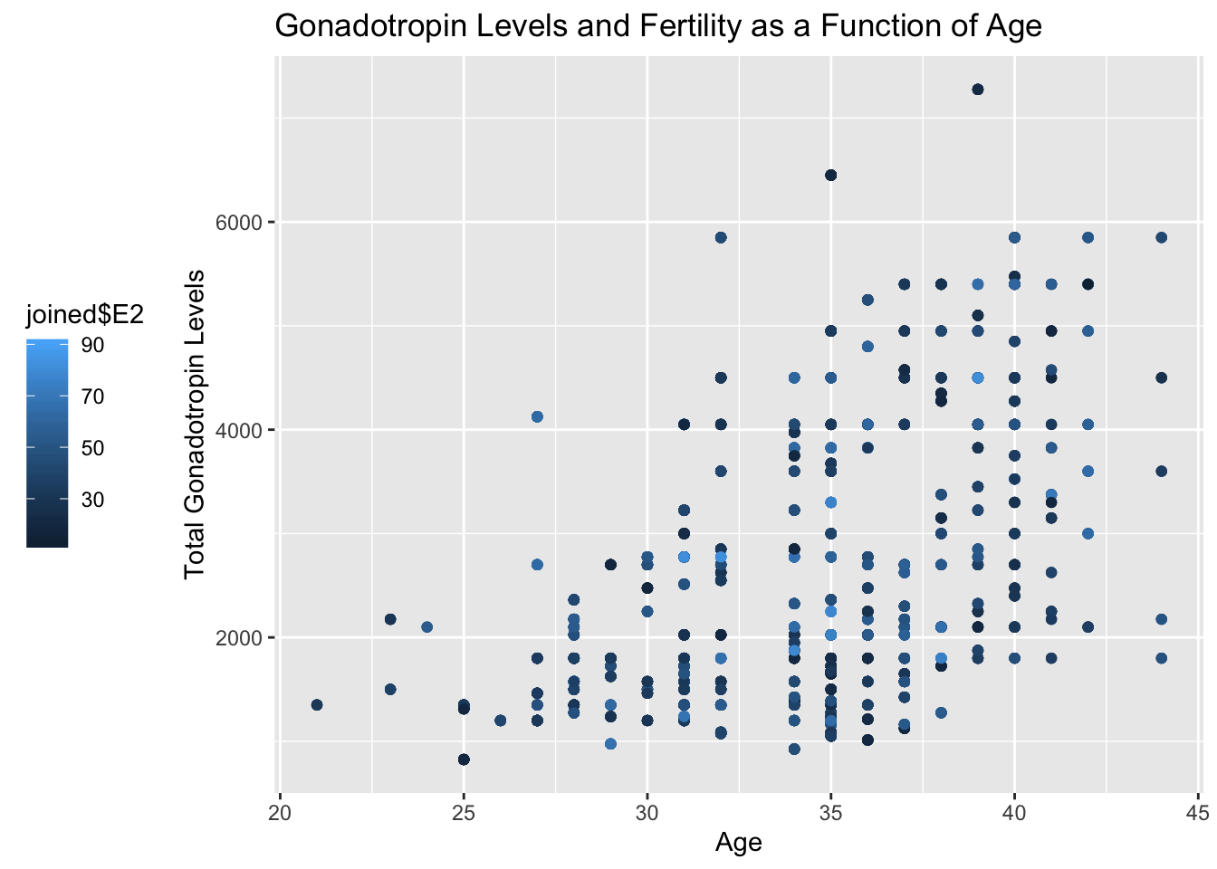
ggplot(data=joined, aes(x=joined$age, y=joined$TotalGn, color=joined$E2)) + geom_point() + ggtitle("Gonadotropin Levels and Fertility as a Function of Age") + xlab("Age") + ylab("Total Gonadotropin Levels") + theme(legend.position = "left")
ggplot(data=joined, aes(x=education, y=LowAFC)) + geom_bar(aes(y=LowAFC, fill = education), stat = "summary", fun.y= "mean") + scale_y_continuous(name = "Antral Follicle Count", breaks = c(0,25,50)) + geom_errorbar(fun.data='mean_se', stat = "summary", width = 0.2) + ggtitle("Antral Follicle Count per Education Level") + scale_fill_hue(h=c(0,40)) + geom_point(aes(y=MeanAFC), stat = "summary", fun.y= "mean", color = "brown")
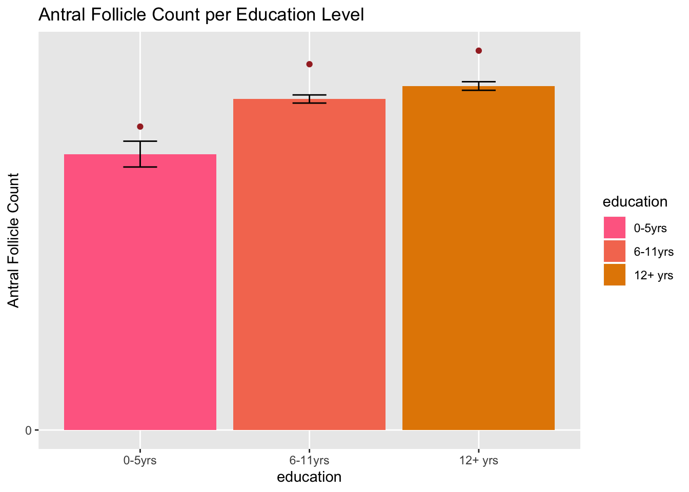
#In my first graph, I used a scatterplot to plot Total Gonadotropin Levels against Age, using fertility as a third variable. Unfortunately, I was expecting to see the gonadotropin levels go down with age as they are necessary for reproduction, as well as seeing fertility levels positively correlated with the gonadotropin levels and negatively correlated with age. The x axis is age, the y axis is total gonadotropin levels and the legend shows the colors and their respective fertility level. In my second graph, I used a bar plot to plot my categorical variable, education along my x axis and my antral follicle count against my y axis. The bars on my graph show the smallest antral follicle count and the third variable, indicated by the red points above the error bars represent the mean antral follicle point.
PCAjoined <- joined %>% dplyr::select(-parity,-education, -FSH, -Oocytes)
joined_nums <- joined %>% select_if(is.numeric) %>% scale
rownames(joined_nums) <- joined$Name
joined_pca <- princomp(na.omit(joined_nums), cor = TRUE, scores = TRUE)
names(joined_pca)
## [1] "sdev" "loadings" "center" "scale" "n.obs" "scores" "call"
summary(joined_pca, loadings = T)
## Importance of components:
##                           Comp.1    Comp.2    Comp.3     Comp.4     Comp.5
## Standard deviation     1.9347389 1.4169340 1.2703162 1.25752207 1.17930928
## Proportion of Variance 0.2339509 0.1254814 0.1008565 0.09883511 0.08692315
## Cumulative Proportion  0.2339509 0.3594323 0.4602887 0.55912384 0.64604699
##                            Comp.6     Comp.7     Comp.8     Comp.9    Comp.10
## Standard deviation     1.14127894 0.97563482 0.90829765 0.82618986 0.80885210
## Proportion of Variance 0.08140735 0.05949146 0.05156279 0.04266185 0.04089011
## Cumulative Proportion  0.72745435 0.78694580 0.83850859 0.88117045 0.92206055
##                          Comp.11    Comp.12    Comp.13   Comp.14     Comp.15
## Standard deviation     0.7126188 0.50712151 0.45338767 0.3724664 0.295644050
## Proportion of Variance 0.0317391 0.01607326 0.01284752 0.0086707 0.005462838
## Cumulative Proportion  0.9537996 0.96987291 0.98272044 0.9913911 0.996853975
##                            Comp.16
## Standard deviation     0.224357746
## Proportion of Variance 0.003146025
## Cumulative Proportion  1.000000000
##
## Loadings:
##                Comp.1 Comp.2 Comp.3 Comp.4 Comp.5 Comp.6 Comp.7 Comp.8 Comp.9
## age            -0.238  0.333        -0.182                0.194  0.144
## parity                 0.139 -0.613  0.138  0.291  0.129         0.379
## induced                      -0.289  0.290  0.548  0.238        -0.463
## case                         -0.424 -0.218 -0.315 -0.198        -0.682
## spontaneous           -0.125 -0.546 -0.297 -0.329 -0.160         0.293
## stratum         0.116 -0.478  0.199 -0.422  0.155  0.150
## pooled.stratum  0.134 -0.452 -0.124 -0.353  0.318  0.235         0.128
## LowAFC          0.369  0.174               -0.248  0.450  0.217
## MeanAFC         0.354  0.182               -0.249  0.471  0.235
## FSH            -0.308               -0.186         0.193 -0.110        -0.672
## E2                    -0.113         0.133  0.104 -0.337  0.880 -0.120
## MaxE2           0.268  0.188        -0.177  0.191 -0.297               -0.617
## MaxDailyGn     -0.402  0.182        -0.286         0.151  0.147         0.187
## TotalGn        -0.402  0.183        -0.277         0.170  0.148         0.149
## Oocytes         0.298  0.352        -0.296  0.207 -0.163                0.148
## Embryos         0.262  0.332        -0.309  0.242 -0.193                0.267
##                Comp.10 Comp.11 Comp.12 Comp.13 Comp.14 Comp.15 Comp.16
## age             0.768  -0.340           0.140
## parity                                 -0.495  -0.300
## induced                                 0.496
## case            0.183                  -0.349
## spontaneous    -0.153                   0.591
## stratum         0.128                          -0.681
## pooled.stratum                         -0.134   0.655
## LowAFC                                                         -0.708
## MeanAFC                                                         0.691
## FSH            -0.386  -0.449
## E2             -0.151  -0.146
## MaxE2           0.180   0.556   0.108
## MaxDailyGn     -0.117   0.341                           0.701
## TotalGn        -0.159   0.346                          -0.702
## Oocytes                -0.182  -0.744
## Embryos        -0.262  -0.268   0.636
eigval<-joined_pca$sdev^2
varprop=round(eigval/sum(eigval),2)
ggplot()+geom_bar(aes(y=varprop,x=1:16),stat="identity")+xlab("")+geom_path(aes(y=varprop,x=1:16))+geom_text(aes(x=1:16,y=varprop,label=round(varprop,2)),vjust=1,col="white",size=3)+scale_y_continuous(breaks=seq(0,.6,.2),labels = scales::percent)+scale_x_continuous(breaks=1:10)
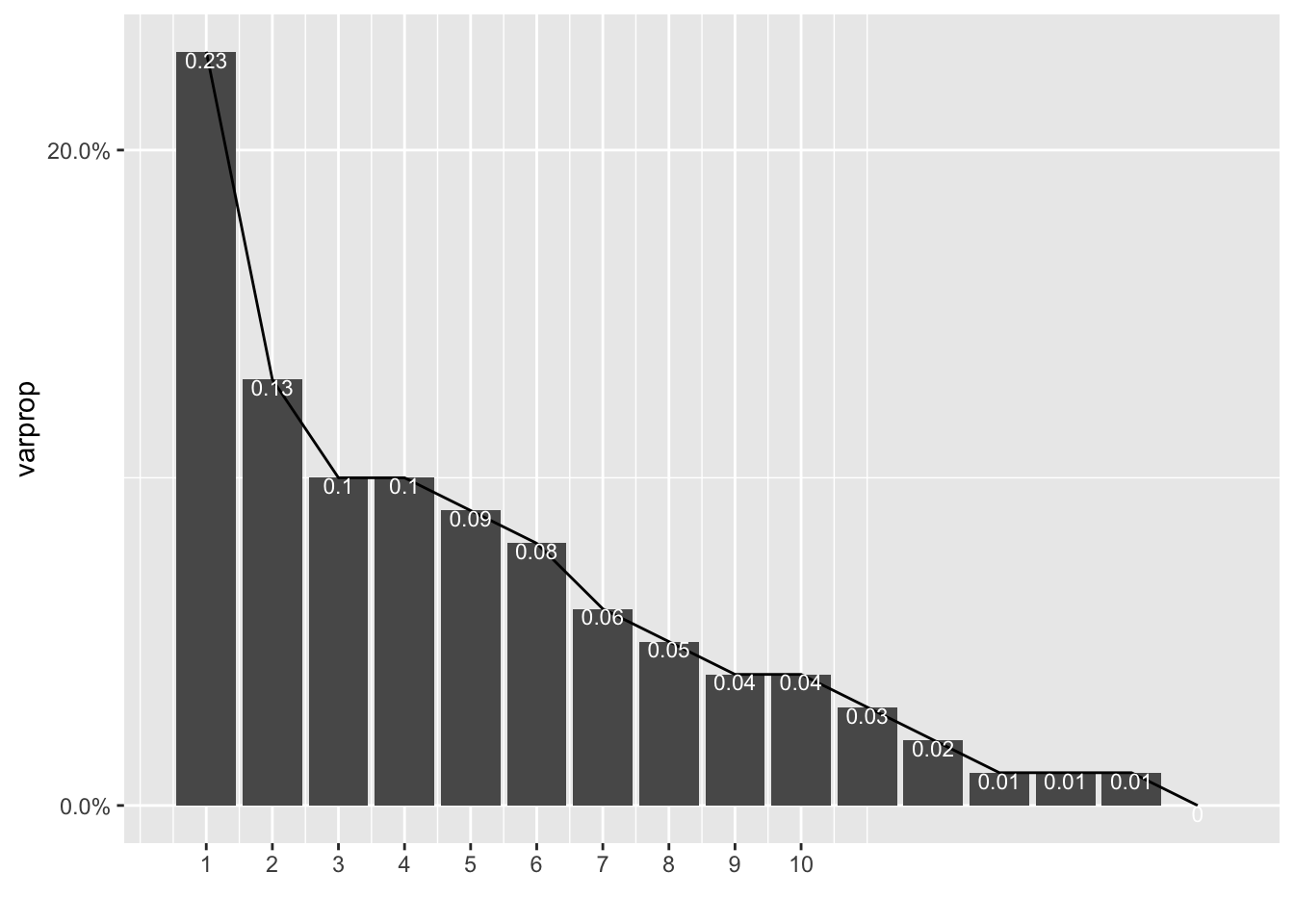
round(cumsum(eigval)/sum(eigval),2)
##  Comp.1  Comp.2  Comp.3  Comp.4  Comp.5  Comp.6  Comp.7  Comp.8  Comp.9 Comp.10
##    0.23    0.36    0.46    0.56    0.65    0.73    0.79    0.84    0.88    0.92
## Comp.11 Comp.12 Comp.13 Comp.14 Comp.15 Comp.16
##    0.95    0.97    0.98    0.99    1.00    1.00
eigval
##    Comp.1    Comp.2    Comp.3    Comp.4    Comp.5    Comp.6    Comp.7    Comp.8
## 3.7432145 2.0077020 1.6137033 1.5813618 1.3907704 1.3025176 0.9518633 0.8250046
##    Comp.9   Comp.10   Comp.11   Comp.12   Comp.13   Comp.14   Comp.15   Comp.16
## 0.6825897 0.6542417 0.5078255 0.2571722 0.2055604 0.1387312 0.0874054 0.0503364
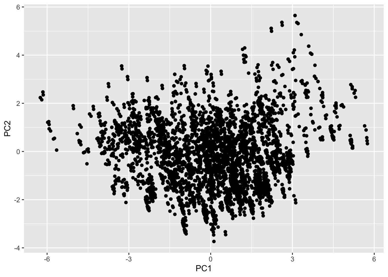
ggplot()+geom_point(aes(joined_pca$scores[,1], joined_pca$scores[,2]))+xlab("PC1")+ylab("PC2")
joined_pca$loadings[1:15,1:2]%>%as.data.frame%>%rownames_to_column%>%
  ggplot()+geom_hline(aes(yintercept=0),lty=2)+
  geom_vline(aes(xintercept=0),lty=2)+ylab("PC2")+xlab("PC1")+
  geom_segment(aes(x=0,y=0,xend=Comp.1,yend=Comp.2),arrow=arrow(),col="red")+
  geom_label(aes(x=Comp.1*1.1,y=Comp.2*1.1,label=rowname))

#The PCA graph and the spacing arrows of the graph shows the correlation between variables and the strength of the correlation. The graph shows us that age and TotalGn indeed do point in the same direction, but unfortunately E2 is in the opposite direction. The PC score plot shows that there is no correlation between PC1 and PC2. Most data seems to be concentrated in the middle where PC1 is between 3 and -3.
Related Posts